HW6

Creating Fake Data Sets To Explore Hypotheses

I’m creating a fake data set on the effects of dolphin watching activities on dolphin behaviour. This can be done by quantifying the occurrence of avoidance responses, one of which is a change in the dolphin’s swimming direction. In this homework I will test the occurrence of directional changes in two conditions: no tourist boats present (control) and with tourist boats present. Based on this, I hypothesise that dolphins will show a greater number of directional changes in the presence of tourist boats.

# Specify parameters
n_no_boats <- 50  # Sample size for the group without boats (number of dolphins)
mean_no_boats <- 9  # Mean of occurrences of directional changes in the group without boats
var_no_boats <- 10   # variance for the group without boats

n_boats <- 50  # Sample size for the group with boats
mean_boats <- 20  # Mean of occurrences of directional changes in the group with boats
var_boats <- 15  # variance for the group with boats

# Generate random data
No_boats <- round(rnorm(n_no_boats, mean = mean_no_boats, sd = sqrt(var_no_boats)),0)
boats <- round(rnorm(n_boats, mean = mean_boats, sd = sqrt(var_boats)),0)

# Combine data into a data frame
data <- data.frame(
  Directional_changes = c(No_boats, boats),
  Group = rep(c("No_boats", "boats"), each = n_no_boats)
)
head(data)

##   Directional_changes    Group
## 1                   5 No_boats
## 2                  14 No_boats
## 3                   5 No_boats
## 4                   9 No_boats
## 5                  16 No_boats
## 6                  12 No_boats

str(data)

## 'data.frame':    100 obs. of  2 variables:
##  $ Directional_changes: num  5 14 5 9 16 12 8 6 11 9 ...
##  $ Group              : chr  "No_boats" "No_boats" "No_boats" "No_boats" ...

Analyzing the data

library(ggplot2)
#ANOVA analysis
anova_result <- aov(Directional_changes ~ Group, data = data)
summary(anova_result)

##             Df Sum Sq Mean Sq F value Pr(>F)    
## Group        1   2927  2926.8   207.7 <2e-16 ***
## Residuals   98   1381    14.1                   
## ---
## Signif. codes:  0 '***' 0.001 '**' 0.01 '*' 0.05 '.' 0.1 ' ' 1

# Generate a boxplot to visualize the data
library(ggplot2)

ggplot(data, aes(x = Group, y = Directional_changes, fill = Group)) +
  geom_boxplot() +
  theme_minimal() +
  labs(
    x = "Group",
    y = "Number of directional changes"
  ) 

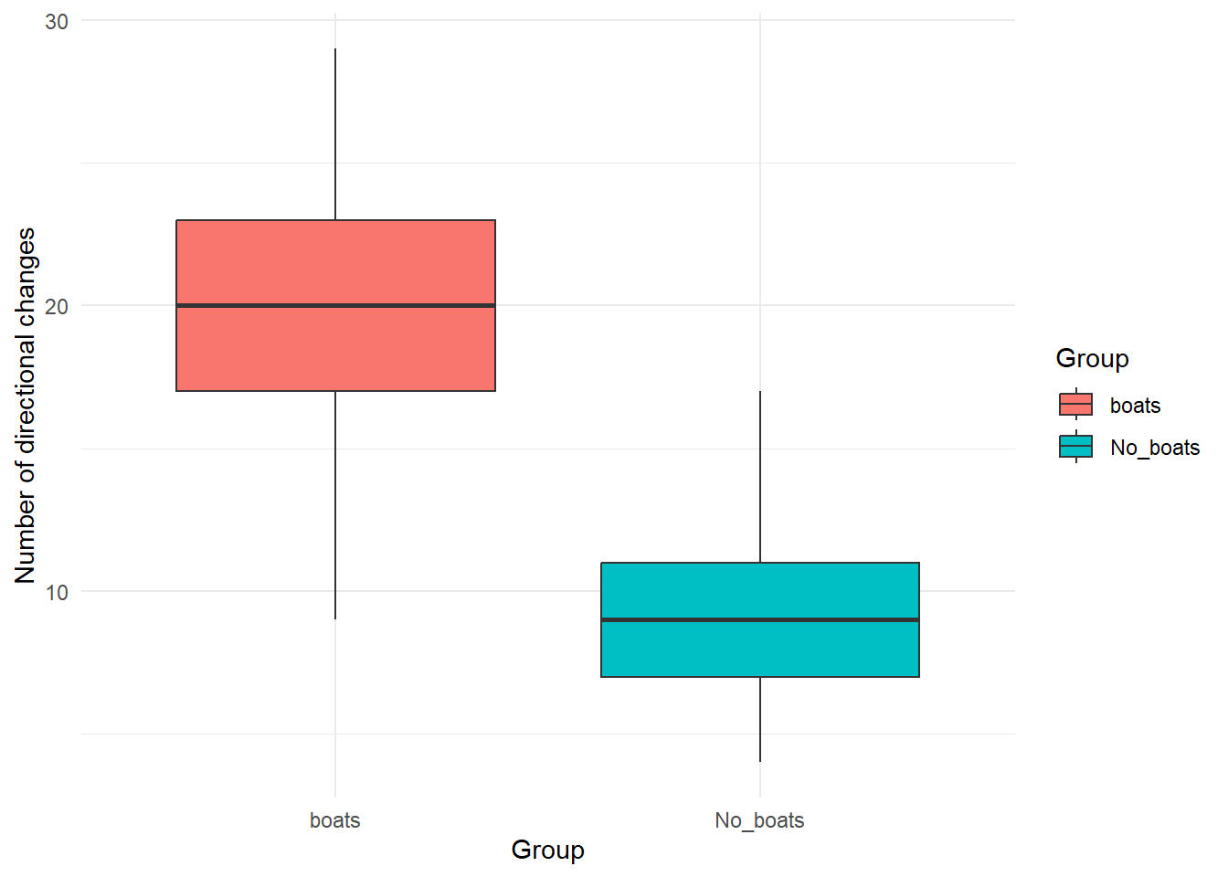##### Using a for loops to adjust the parameters and explore how they might impact the results/analysis.How small can your sample size be before you detect a significant pattern (p < 0.05)? How small can the differences between the groups be (the “effect size”) for you to still detect a significant pattern?

library(dplyr)

## 
## Adjuntando el paquete: 'dplyr'

## The following objects are masked from 'package:stats':
## 
##     filter, lag

## The following objects are masked from 'package:base':
## 
##     intersect, setdiff, setequal, union

#variables to explore
effect_sizes <- seq(1, 10, 0.5)  # Varying effect sizes
sample_sizes <- seq(5, 50, 5) # Varying sample sizes
alpha <- 0.05

# data frame to store the results
sample_size_results <- data.frame()
# creating the loop
for (effect in effect_sizes) {
  for (n in sample_sizes) {
    group_boats <- rnorm(n, mean = mean_boats, sd = sqrt(var_boats))
    group_no_boats <- rnorm(n, mean = mean_no_boats + effect, sd = sqrt(var_no_boats))
    t_test <- t.test(group_boats, group_no_boats)
    p_value <- t_test$p.value
    # storing the results
    sample_size_results <- rbind(sample_size_results, 
                     data.frame(Effect_Size = effect, 
                                Sample_Size = n, 
                                P_Value = p_value, 
                                Significant = (p_value < alpha)))
  }
}

# View the first few rows of results
print(head(sample_size_results))

##   Effect_Size Sample_Size      P_Value Significant
## 1           1           5 5.119420e-03        TRUE
## 2           1          10 2.046770e-04        TRUE
## 3           1          15 1.670127e-07        TRUE
## 4           1          20 3.299073e-10        TRUE
## 5           1          25 4.654102e-12        TRUE
## 6           1          30 1.809820e-16        TRUE

# filtering the data frame for significant results with small sample sizes
sample_size_results %>% filter(Significant == TRUE & Sample_Size <= 5)

##   Effect_Size Sample_Size      P_Value Significant
## 1         1.0           5 0.0051194196        TRUE
## 2         1.5           5 0.0342455382        TRUE
## 3         2.0           5 0.0001913736        TRUE
## 4         2.5           5 0.0234802309        TRUE
## 5         4.0           5 0.0023766565        TRUE
## 6         5.0           5 0.0158632797        TRUE
## 7         5.5           5 0.0062711853        TRUE
## 8         6.0           5 0.0054363660        TRUE

The table above shows that the minimum sample size to see significant differences between groups is 5, and a differences of 1 between means is enough to still see a difference.